15 Useful Google Sheets Formulas That Can Make Work Easier

Google Sheets is a versatile spreadsheet app you can use across multiple platforms, including any browser as a web app, on Android or iOS as a mobile app, or even as a desktop app through ChromeOS. Because it's web-based and cloud-based, Sheets is a great collaborative tool to use with remote teams especially, but there are plenty of Sheets tips and tricks to increase productivity for personal projects as well.

Whether you're using Google Sheets for small business templates or to create the perfect personal budget for your family, knowing how to use formulas in the app will improve your experience tenfold.

Instead of manually calculating totals, copying and pasting data, or typing in data rather than importing it, use formulas to save a ton of time and energy. To use any of the formulas mentioned here, simply type an equal sign (=) followed by the name of the formula. With that, let's jump into 15 of the most useful Google Sheets formulas you can use to make work easier.

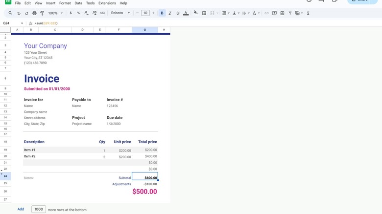
Type an equal sign (=) followed by "SUM" to automatically total everything in a single row or column in Sheets. You can manually type (G19:G23) — or whichever cells you're trying to add — or simply press enter after typing SUM, click and drag to select your range, and press enter again to complete the formula.

This is a helpful formula to have on hand, whether you're totaling up line items for an invoice, a daily sales total, or personal expenses for a budget. Plus, after you have the SUM formula set up, the cell it's in will update automatically when you change any number within the specified range.

It's worth noting you don't have to use a single column or row with this function. If you need to get the sum of multiple random cells — like F19, G19, and G25, for example — you just need to type =SUM(F19, G19, G25). For more advanced Sheets users, check out the SUMIF function for totaling within certain parameters.

The XLOOKUP formula is a more advanced version of old classics like VLOOKUP and HLOOKUP, and it functions quite similarly. This formula is useful for searching through a large database for a specific value. XLOOKUP allows you to search both horizontally or vertically, whereas VLOOKUP only searches vertically and HLOOKUP only searches horizontally.

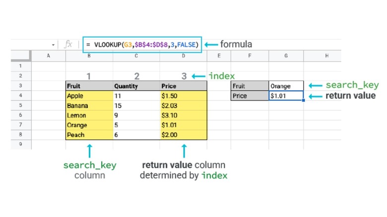
Here's the syntax for this formula: XLOOKUP(search_key, lookup_range, result_range, missing_value, match_mode, search_mode). The search key is the value you're trying to search for, put in its own designated cell on your sheet. The lookup range is the column or row you want to search in, and the result range is the column or row you want your corresponding result to be pulled from.

The last three arguments in this formula are completely optional if you need to further narrow or customize your search. For simple searches, a completed formula may look like this: =XLOOKUP("Orange", B4:B8, D4:D8).

By typing an equal sign (=) followed by the function name "COUNT," you can quickly tally up how many numerical values there are within the data you're looking at. This can be helpful for keeping track of sales, ensuring surveys are filled out completely, or seeing how many data values you need to pay attention to when creating charts, graphics, or a presentation.

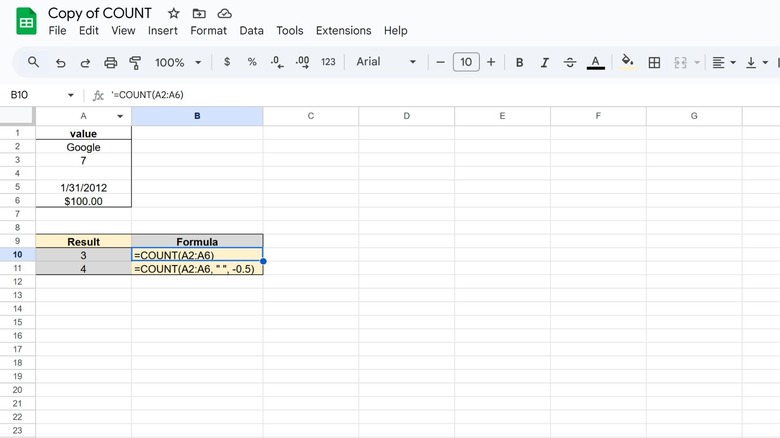
The syntax is super simple for this formula. Here's an example of the formula in action: =COUNT(A2:A6). It will automatically search cells A2 through A6 for numerical values, ignoring any cells that are either empty or contain text.

If you want to get more specific with a tally, you can use the COUNTIF formula instead. After specifying the search range, you'd add a search term in quotation marks. For instance, you could type =COUNTIF(A2:A6, "1/31/2012") to search for the number of cells containing that exact date entry.

Use the AVERAGE formula in Google Sheets to, as the name suggests, average a set of numerical values. While this can be simple to do with only a few numbers via manual calculation or mental math, it gets much trickier when you're dealing with a large set of numbers or complicated amounts with decimal points.

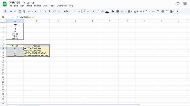
By using the formula =AVERAGE(A2:A4) in the image above, it'll automatically add 2, -1, and 11 together to get 12, and then divide by 3 to get the average. Seeing it work with just three numbers, isn't that impressive. But imagine using this formula to average the total of 30 takeout totals to see how much you're spending per meal every time you go out to eat — suddenly, the value of this simple formula goes way up.

This is also a great formula for teachers to average grades, for other budget-related uses, and for identifying common trends in large data sets.

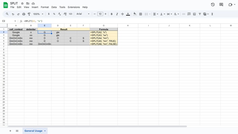
The SPLIT formula in Sheets is helpful for separating out data so it's much easier to look at or sort, especially when it's imported from another source. When data is imported to Sheets, sometimes it all ends up in a single column, with names, addresses, phone numbers, and more separated by commas or spaces.

You can use the split formula with a comma as a delimiter, or a character that separates text strings, to automatically sort a ton of different information into multiple columns. Targeting rows A2 through A10, that formula would look like this: =SPLIT(A2:A10, ",").

Here's the syntax for the SPLIT formula in Google Sheets: SPLIT(text, delimiter, [split_by_each], [remove_empty_text]). The last two arguments in brackets at the end of the formula are both optional and true by default. They're only there to help you further customize and narrow down how to divide the text you're looking at.

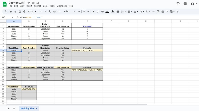
Whether you're working on a personal budget, planning your wedding, or tackling data-intensive tasks for work, the SORT formula in Sheets makes organizing and filtering data much easier. You can import data from another source or manually type all the info you need, and then sort it alphabetically, numerically, and in ascending or descending order.

To select a range of rows and columns, enter the cell at the top left of the range and the cell at the bottom right of the range, with a colon separating the two cell identifiers. For example, the range A2:D6 would select all columns and rows that would be highlighted if you dragged your cursor from cell A2 to cell D6.

Typing =SORT(A2:D6, 2, TRUE) will sort your data in ascending order, from the smallest value to the largest (or A to Z). Swapping out TRUE for FALSE will sort your data in descending order. To sort more specifically, check out the FILTER formula.

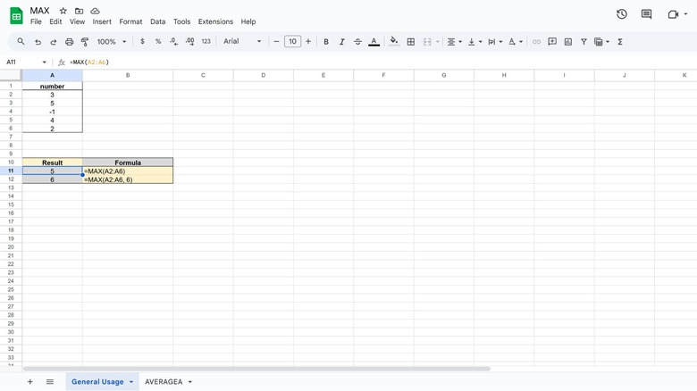
Another simple, yet incredibly helpful formula to use in Google Sheets is =MAX or =MIN. Using these two formulas will deliver the maximum and minimum numeric value within a dataset, respectively.

In a purely professional setting, these formulas can assist with sifting through massive amounts of data to find the highest or lowest sales figure, who in the company has the best service rating, or which tasks take the longest amount of time to complete.

When it comes to personal use, MAX and MIN formulas can help with creating insightful budgets. For those just starting to create a budget, it is generally advised to keep track of every single dollar you spend for a month or two. If you keep track in Google Sheets, you can quickly find out what you spend the most and least on, making it much easier to stick to a budget over time.

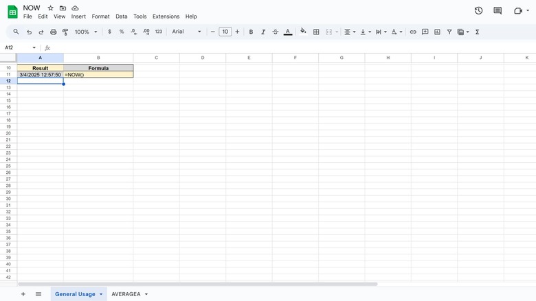
This is perhaps one of the most basic formulas you can use in Google Sheets, but that doesn't make it any less useful. By simply typing =NOW() in a cell, Sheets will automatically grab the current date and time and display it. Every time you open the Sheet or refresh the page, the cell with the NOW formula will update to the current date and time. It's like having a built-in clock in your Sheet, helpful if you have your taskbar hidden to give you more screen real estate on the daily.

You can also use the NOW formula to create easy-to-use timestamps if you need to track your hours worked. Use NOW to pull the exact day and time you're starting work, copy and paste that value somewhere else, and refresh the Sheet when you're finished working to get an end timestamp.

On a similar note, typing =TODAY() will automatically populate the current date without the time, helpful for creating invoices, memos, or other documents that need to track the current day.

If you ever need to go back and fix a spelling mistake or another major text error that occurs multiple times in Google Sheets, don't fix the mistakes manually. Instead, utilize the handy SUBSTITUTE formula.

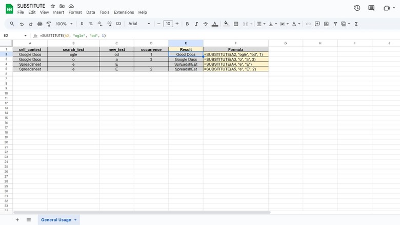
Here's the syntax for this formula: SUBSTITUTE(text_to_search, search_for, replace_with, [occurrence_number]). Inputting an occurrence number at the end is entirely optional and only needed if you want to replace a specific instance rather than all of the instances throughout the Sheet.

First, you need to identify "text_to_search," or the text you want the formula to search. This can also be a cell reference instead of a text string. Then, list the text or string you want to replace in the "search_for" slot, and the text you want to replace it with in the "replace_with" slot. In a simple example, here's the formula you'd use to replace "world" with "globe" in the phrase "Hello world": =SUBSTITUTE("Hello world", "world", "globe"). This way, you can replace text just as easily as you can in Google Docs with the help of a built-in tool to find and replace words, phrases, and symbols.

Whether you're working with grades, amounts of money, or other data values, using the ROUND formula in Google Sheets can help keep all your info neat and organized. As the name implies, this formula automatically rounds the numbers or cells you provide to the number of places you set.

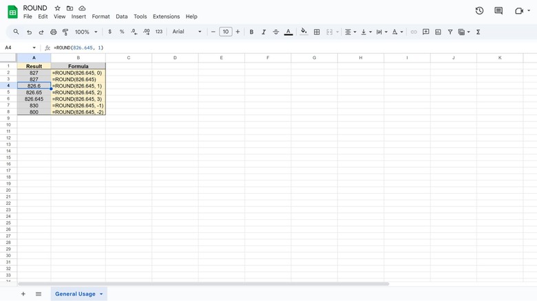
The formula's syntax is quite simple: ROUND(value, [places]). If you don't specify a number of places to round to after the decimal point, the formula defaults to zero places or a whole number.

What's nice about this formula is that you get to keep the true recorded value in case you need to know what the full number is, but on the surface, it'll appear rounded to your preference. For example, if you want to see rounded numbers for ease and tax purposes, you can set your visual preference to that, but any time you click on a cell, you can see the specific dollar amounts you first entered.

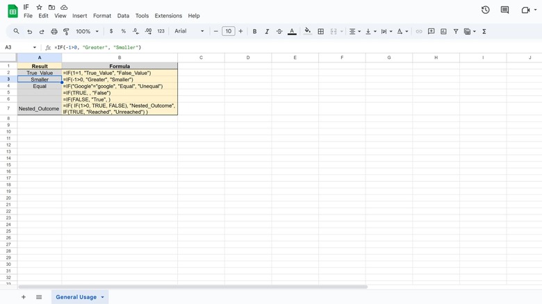
Using the IF formula in Google Sheets is a little more complicated than some of the other formulas mentioned, but once you get the hang of it, it'll become second nature and muscle memory. The syntax for this formula is: IF(logical_expression, value_if_true, value_if_false).

The logical expression is the "if" part of your condition, followed by what value it should return if the statement is true (value_if_true), and then the value it should return if the statement is false (value_if_false). This can be helpful for teachers assigning letter grades based on numerical scores, managing inventory levels, or identifying top-performing employees based on certain tracked performance metrics.

For a teacher assigning pass or fail grades, an IF formula may look like this: =IF(B3>69.5, "Pass", "Fail"). You can also write multiple IF formulas within one, using parentheses, making it possible to assign specific letter grades based on numerical ranges or customized outcomes.

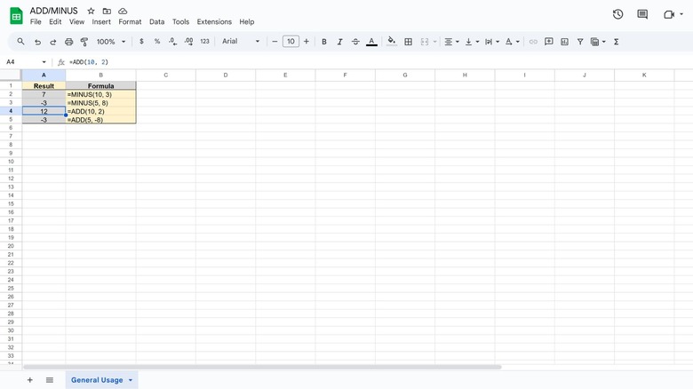
These are two more formulas in Google Sheets that do exactly what their names suggest. When you type =ADD(2, 3), the cell will return the sum of 5. If you type =MINUS(2, 3), the cell will read -1 instead. You can add as many numbers as you need, as long as they're separated by commas.

Rather than opening a separate calculator app on your phone or computer, you can do simple calculations directly in Sheets. Just pick any empty cell in your file and enter the formula and the numbers you need added or subtracted.

To make things faster, you don't need to fully type ADD or MINUS. Instead, after typing an equal sign (=), type the numbers you need to add or subtract separated by a plus sign (+) or a minus sign (-). For example, typing =2+3 in an empty cell will automatically give you a sum of 5.

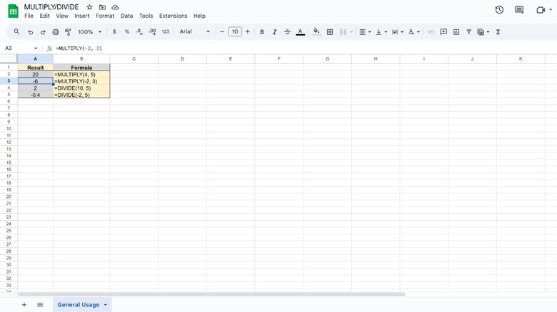
Just like you can use ADD and MINUS to perform simple addition and subtraction in Google Sheets, you can use MULTIPLY and DIVIDE to handle basic multiplication and division. Anything you can do to stay in your Sheets file, like ditching a separate calculator app, will help you work faster and be more productive overall.

There are two ways you can multiply numbers in Sheets. Either type =MULTIPLY followed by the numbers you want to multiply inside parentheses and separated by commas, like =MULTIPLY(4, 5), or you can format it with an asterisk (*) like this: =4*5. Either way, the result will be the same.

Similarly, you can divide using the DIVIDE formula or by using an equal sign (=), a forward slash (/), and the numbers you're trying to divide. For example, you'll get the same results by typing =DIVIDE(20, 5) and =20/5 in an empty cell.

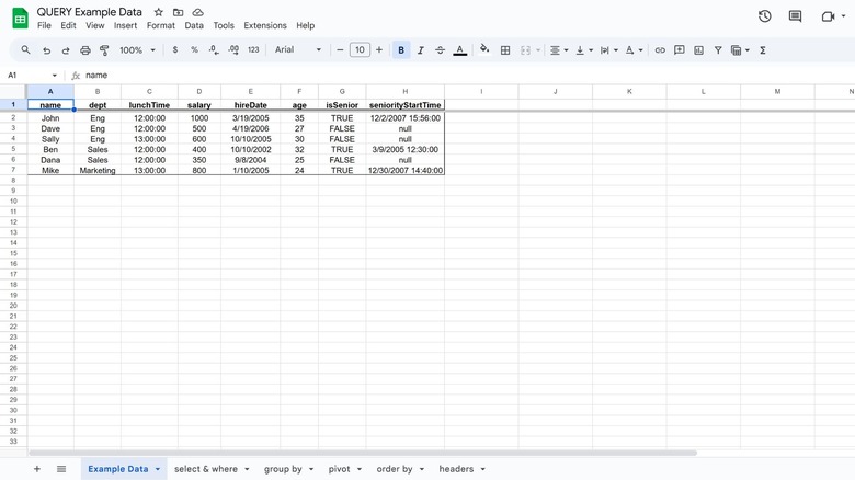
Although the QUERY function can be tricky to master for budding Google Sheets users, it's an incredibly powerful tool to have in your arsenal, much like these tips for getting the most out of Google Drive.

Here's the formula's syntax: QUERY(data, query, [headers]). "Data" refers to the range of cells you're looking to analyze, "query" plainly refers to the query you're trying to run, and "[headers]" is an optional number you can add to state the number of header rows in your data range.

Using the QUERY formula with a few query-specific keywords — like Select, Where, Group by, and others — lets you easily look through a massive data set for just the information you need. It can also be a great way to approach a large data set from different perspectives. If you need help figuring out where to start when creating your own query, Google has an extensive doc on query language you can follow.

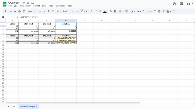
One of the most unexpected uses for Google Sheets that's incredibly helpful is the CONVERT formula. With a built-in database of multiple conversion units, Sheets is capable of converting inches to feet, seconds to minutes, Celsius to Fahrenheit, and so much more.

Whether you're working on creating a virtual cookbook and need to convert U.K.-based recipes to U.S.-based measurements or another similarly intensive project with lots of conversions, or you simply want to perform a quick conversion in Sheets without needing to open a new tab to search, the CONVERT formula will prove its usefulness quickly.

Here's the syntax: CONVERT(value, start_unit, end_unit). You do need to be specific with how the unit is abbreviated, based on what Google has specified in the extensive list of conversion units available via Sheets, and make sure to put the units in quotation marks. For example, =CONVERT(12, "in", "ft") would result in an answer of 1, but =CONVERT(12, "inches", "feet") would result in an error.