What Is The Lookup Function In Excel & How Do You Use It?

While using Microsoft Excel for data analysis, you may sometimes need to search for and retrieve specific values. In such cases, Excel's LOOKUP function can be extremely useful. It allows you to search for a value in a range of cells and return a corresponding value from another range. This function is especially helpful when you're working with large datasets, where manually searching for values would be inefficient and time-consuming.

The basic LOOKUP function in Excel comes in two forms: vector lookup and array lookup. The vector form searches for a value in a single row or column and returns a corresponding value from another row or column, while the array form works with larger table-like data ranges. There are also advanced Excel functions like VLOOKUP, HLOOKUP, and XLOOKUP that provide more advanced lookup functions that offer greater flexibility and improved accuracy.

In this article, we'll explain how the LOOKUP function works, along with examples. We'll also explore VLOOKUP, HLOOKUP, and XLOOKUP to help you use them effectively in Excel. Let's get started!

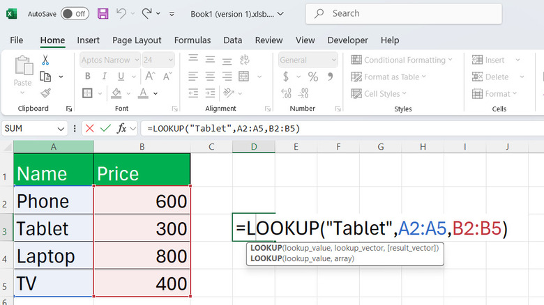
Using the LOOKUP function in vector form allows you to search for a value in a single row or column and retrieve a corresponding value from another row or column of the same size. The syntax for the LOOKUP function in vector form is: LOOKUP(lookup_value, lookup_vector, result_vector). Here, "lookup_value" is the value being searched for, "lookup_vector" is the range where Excel searches for the value, and "result_vector" is the range from which the corresponding value is retrieved. 

For example, suppose you have a list of products in column A (A2:A5) and their corresponding prices in column B (B2:B5), as shown in the above image. If you want to find the price of a particular product like "Tablet," you can use the following formula: =LOOKUP("Tablet", A2:A5, B2:B5). In this case, Excel will search for "Tablet" within the lookup range (A2:A5) and return the corresponding price from the result range (B2:B5).

Note that the LOOKUP function performs an approximate match. In other words, it first searches for an exact match, and if it does not find one, it returns the largest value in the lookup vector that is less than or equal to the lookup value. However, if the lookup value is smaller than the smallest value in the lookup vector, the function will return a #N/A error.

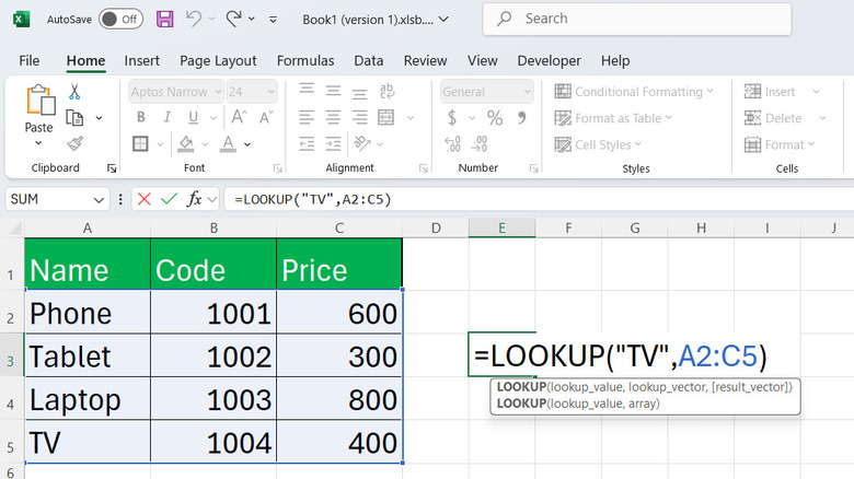
The array form of the LOOKUP function is useful for large datasets organized in a rectangular range with multiple rows or columns. It searches for a value in the first row (for horizontally arranged data) or the first column (for vertically arranged data) of the specified array and returns a corresponding value from the last row or column. The syntax for using the LOOKUP function in array form is: LOOKUP(lookup_value, array). Here, "lookup_value" refers to the value you wish to find, while "array" indicates the dataset where the lookup should be performed. 

For instance, consider a dataset where column A (A2:A5) contains product names, and column C (C2:C5) lists their prices. If you want to determine the price of a specific product, such as "TV," you can use this formula: =LOOKUP("TV", A2:C5) This function first will search for "TV" in column A (the first column of the array). Once it locates the value, it will retrieve the corresponding data from the last column of the specified array, which is column C, returning the price of the TV. 

While the LOOKUP function is useful for quick searches, it requires your data to be arranged in ascending order for accurate results. For greater flexibility and more advanced options, it's better to use Excel's VLOOKUP, HLOOKUP, or XLOOKUP functions.

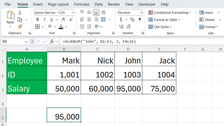
Excel's HLOOKUP (Horizontal Lookup) function can search for a value in the first row of a table and then return a value in the same column from a row you specify. The syntax for HLOOKUP is: =HLOOKUP(lookup_value, table_array, row_index_num, [range_lookup]) Here, "lookup_value" is the value to find, "table_array" is the dataset where the search is performed, and "row_index_num specifies" the row number from which to return the corresponding value. The "[range_lookup]" argument is optional and determines whether the match should be exact (FALSE) or approximate (TRUE).

For example, if you have a list of employees in row 1 and their salaries in row 3, as shown in the above image, you can use the following formula to find the salary of a specific employee: =HLOOKUP("John", B1:E3, 3, FALSE) This formula instructs Excel to search for "John" in row 1 and return his corresponding salary from row 3. If an exact match is not found, the function returns a #N/A error (unless you use an approximate match).

Excel's VLOOKUP (Vertical Lookup) works similarly but searches for values across columns instead of rows. It is useful when your data is structured vertically, with the lookup values in the first column of a dataset. 

XLOOKUP is the most powerful and flexible lookup function in Excel. Unlike VLOOKUP and HLOOKUP, it can search both vertically and horizontally, supports exact matches by default, and allows searches in both forward and reverse directions. The syntax for XLOOKUP is: =XLOOKUP(lookup_value, lookup_array, return_array, [if_not_found], [match_mode], [search_mode]). Here's what each argument means:

In this formula, "lookup_value" is the value to search for, "lookup_array" is the range where the search occurs, and the "return_array" specifies the range from which to return the corresponding value. The optional "[if_not_found]" argument prevents #N/A errors by displaying a custom message when no match is found, while "[match_mode]" lets you choose the type of match, such as exact, approximate, or wildcard. Finally, the "[search_mode]" allows you to specify the search direction, either top-to-bottom (default) or bottom-to-top for more flexibility.

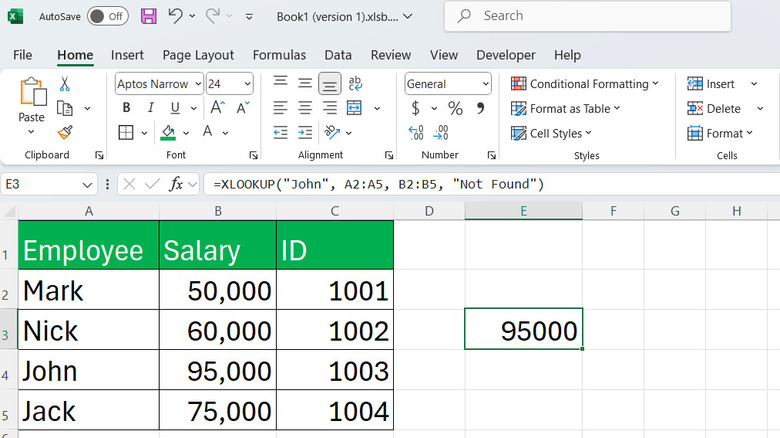
For example, suppose you have a dataset where column A contains employee names and column B contains their salaries. To find a specific employee's salary, you can use: =XLOOKUP("John", A2:A5, B2:B5, "Not Found"). This formula searches for "John" in column A and returns the corresponding salary from column B. If "John" is not found, instead of returning an error, the function displays "Not Found" as specified in the [if_not_found] argument.

Note that XLOOKUP is not available in older versions of Excel, such as Office 2016 and Office 2019. So, you'll need Office 2021, Office 2024, or Microsoft 365. If you're using an older version, you can use VLOOKUP or HLOOKUP instead.