Power Query For Beginners: 6 Commands To Get Started

Excel is a powerhouse at transforming and manipulating data, thanks to a wide variety of Excel formulas and in-app tools. Add Power Query to this already powerful mix, and you get an even more streamlined method to extract data from different sources and transform it on the go. 

If you are a beginner, Power Query can be intimidating at first. It transports you to a completely unfamiliar Excel section with a different user interface and menu options. Moreover, your standard formulas no longer behave the same and a new coding language, M code, comes into the picture. 

That said, once you get past the initial learning curve, Power Query is one of the most effective tools to perform batch transformations on bulk data while keeping complete track of each data manipulation step in the process. Here's a thorough guide on the best commands to get you started with Power Query and building a strong foundation.

Before diving into the commands, let's first understand the fundamentals of Power Query and how it works. While basic Excel lets you create or paste a table in the spreadsheet itself, Power Query can connect to a variety of sources to get the data. That's also why the first step to accessing Power Query is to head to the "Get & Transform Data" section under the "Data" tab and select a data source. Excel supports getting data from multiple data sources such as, databases, webpages, CSVs, Excels, PDFs, and many more file types. A massive perk of using Power Query is the ability to connect and merge multiple data sources into one.

Once you connect your data sources, you can either "Load" or "Transform" this data. Loading data refers to importing the data into an Excel worksheet or Power BI report.

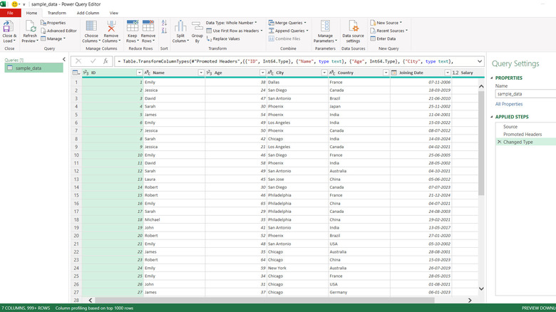
Transforming the data refers to performing data manipulation using the Power Query editor. That's where you can bring all the handy Power Query commands into work. The top of the Power Query editor sports different tabs that integrate all the important features for data manipulation. The left side features the "Query" section, listing all the data sources connected to the editor. The formula bar below the different tabs contains the formula in M language. In the center, you can find a preview of your connected data in a tabular form. The rightmost side contains the "Applied Steps" section, listing all the manipulation steps you perform while transforming the data.

If you are just starting, here are some of the best and most commonly used Power Query commands to get you all geared up.

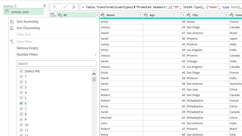
Filtering a column works almost exactly as it would with an Excel worksheet but with added convenience. While Excel makes you first apply filters to your column headers, Power Query has the filters applied by default. To filter a column, click on the dropdown next to the column headers to open the list of all values in the column. Uncheck the values you need to filter out and click OK to complete the filtering.

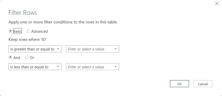
You may also use the text and number filters to filter the value according to predefined rules. For instance, if you need to filter the people aged 18 to 23, you can apply the "Between" filter in the Number Filters tab.

Samyak Goswami

When you apply a filter, the formula bar updates with the corresponding M query. You can also modify the code right from the formula bar to update the filter. Moreover, the filtering process should show as an applied step in the "Applied Steps" section in the editor.

The Split Column feature is an extremely capable tool for dividing columns based on delimiters, number of characters, digits, and even character types. For instance, consider an Excel mailing list with a column containing addresses as – "Address, Zip Code". Now, you want to split the address column into an address and a zip code column

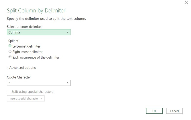
As the "," is the common delimiter for all the values in the Address column, you can split the column using the delimiter. Alternatively, you can also split the zip codes based on the number of characters if your zip code data has a fixed number of characters.

Samyak Goswami

For splitting columns, first click on the column header to select the entire column. Next, click on the Split column option in the Home or Transform tab and select By Delimiter. Specify a delimiter in the dialog box and click OK to split the columns. You should now see two columns named "Address.1" and "Address.2" which you can further rename to Address and Zip Code.

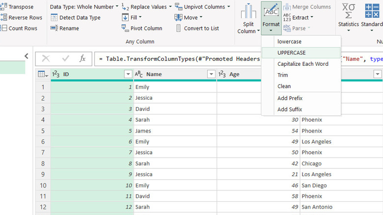
Cleaning and formatting your data is as important as manipulating it to make it visually appealing and consistent. Similar to most of the other commands mentioned on this list, formatting, trimming, and cleaning values follow non-identical approaches in a regular Excel sheet, but Power Query clubs these essential features into a single menu option — Format. The Format feature in the Transform tab allows for Lower Case, Upper Case, and Capitalizing each word with on-the-go buttons

For using the Format option, simply select a column containing text values and go to the Format option. Clicking on lower case or upper case options transforms the entire column to only contain the respective case. Moreover, the Capitalize each word feature essentially works similar to title case in Word, capitalizing the first letter of each word.

Apart from these somewhat basic formatting features, the Format feature offers data Trim and Clean functionalities. If your data contains unwanted spaces between characters in the beginning or end of the cell values, the trim function can automatically remove all these spaces. Moreover, the clean function removes all the unprintable characters from the data, making it fit for printing.

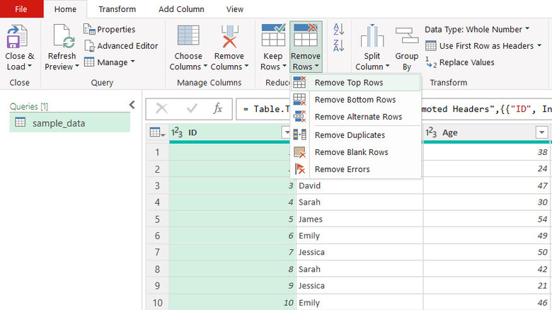
Removing duplicates is a common operation that you need to perform often while transforming data. The "Remove Duplicates" command retains only the first occurrence of each value and removes the rest. Another important operation, "Remove Blanks," refers to eliminating rows containing no values from the data.

In a regular Excel Worksheet, removing duplicates and removing blanks involve following very different methods. Power Query streamlines removing rows from your data based on different criteria and brings it all under one roof. To remove any unwanted row, select a column or bunch of columns from which you want to remove the duplicates. Next, head on to the "Remove Rows" section in the Home tab and click on the dropdown arrow. Now, select the "Remove Duplicates" option, and your selected columns should now only have unique values for each row.

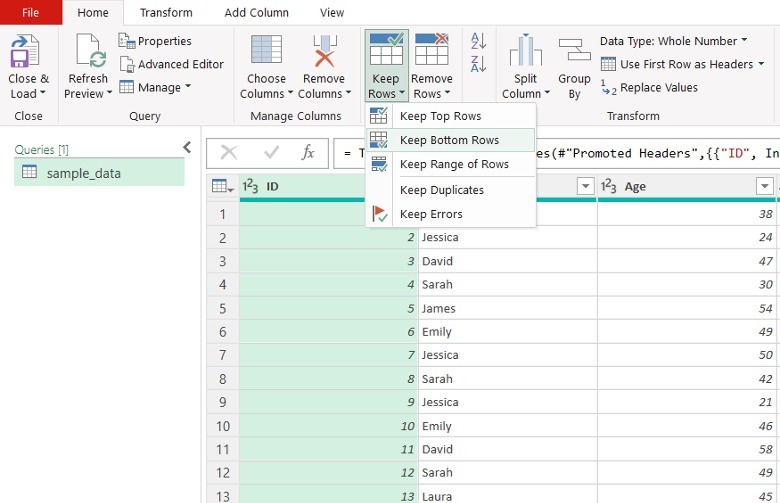
What happens when you need only the duplicate values in your columns? The Power Query editor has a trick up its sleeves to cover you up using the Keep Rows option.

Samyak Goswami

As the name suggests, the "Keep Rows" feature acts exactly opposite to the Remove Rows feature, and you can remove all unique values using the "Keep Duplicates" option.

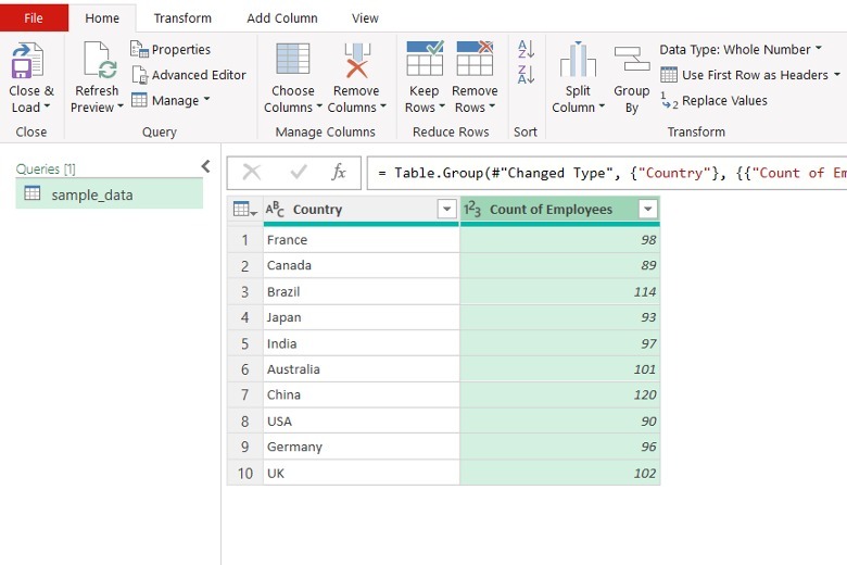
If you are into data analysis, Group By would not be new to you, as it is a fundamental SQL function. Power Query presents this complex yet useful function in a simplified and interactive way using dialog boxes and drop-downs. Group By essentially transforms the data based on one or more columns by reevaluating it for one of the core operations – sum, count, average, median, min, max, and all rows. Although the definition makes it sound no less than rocket science, Group By is a relatively easy command once you get a hold of it. Consider a data containing names, age, country, and salary of different employees from an organization. The problem statement is to depict the number of employees from each country in a basic table containing country name and count of employees. To create this table, click on the Group By option in the Home or Transform Tab and wait for the Group By dialog box.

Now, select the column with which you want to group your data. For the current problem statement, select the "Country" column and select the "Count Rows" operation. Now, rename the new column as "Count of Employees" and hit OK.

Samyak Goswami

This basic Group By operation, involving a single Group By column, is great for grasping the essence of the function, but Power Query offers advanced Group By as well, where you can group multiple columns together and perform more complex operations.

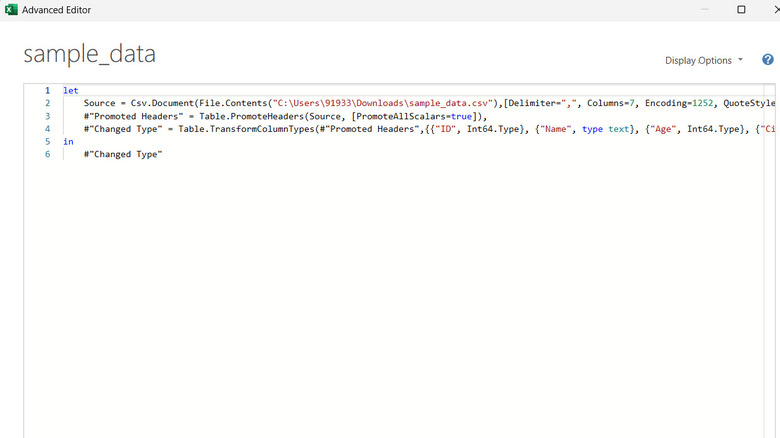
The formula bar in the Power Query Editor updates automatically with the M code corresponding to the applied data manipulation step. The M code can seem intimidating at first, but you can easily get a hold of its syntax after a closer look. The Advanced Editor option in the Home tab opens a condensed M code editor for all the applied steps for a data. You can write the M code directly in this editor to add additional steps to your transformation. That said, using M code to write entire steps can immensely slow down your workflow, especially as a beginner. The best way to use M code is to modify the code to avoid altering steps using the editor interface. Moreover, you can copy and paste similar M codes to perform the same actions in different steps.

The Power Query editor is an extremely powerful tool with a massive array of data transformation features. While these commands should get you a good head start, Power Query can do a lot more with merge functionality that allows cross data-source joining of tables, appending different data sources, and much more.