How To Compare Two Columns In Excel

When it comes to working with data, whether it's a basic list of entries or a large dataset, Excel is usually one of the go-to tools for most people, and for good reasons. First off, it allows you to visualize data in a variety of ways, from simple pie and line charts to more complex sunbursts and treemaps. Its interface is also pretty intuitive even for beginners, and if you get lost, there's always the search bar to help you out.

On top of this, Excel is rich in features for organizing and analyzing data too. You have the option to alphabetize the data in Excel, filter the entries, remove duplicate and blank cells, and even extract specific portions of text from cells. Another handy data analysis feature in Excel is comparing columns, something you'll typically use for things like matching placed orders with fulfilled ones, tracking scheduled versus actual employee attendance, and comparing customer data between two time periods. There are multiple ways to compare two columns in Excel, and in this guide, we'll cover three of these methods.

Conditional formatting is one of the best hacks in Excel, as it lets you highlight key data, making it easier and faster to analyze your sheet at a glance. It typically comes in handy when you need to spot approaching or missed deadlines, track task completion, and display a budget's low and high figures. However, you can also use conditional formatting to compare two columns in Excel. Here's how:

1. Open the Excel spreadsheet containing the columns you want to compare.
2. Select the data in both columns, excluding the heading.
3. In the Styles section in the Home tab, click on Conditional Formatting.
4. Choose Highlight Cells Rules from the drop-down menu.
5. Go to Duplicate Values.
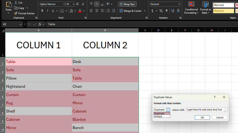
6. To highlight only the items present in both columns, leave the value as Duplicate in the Duplicate Values dialog box.
7. To single out entries that appear in only one column, click on Duplicate and switch to Unique in the dialog box.
8. (Optional) You can change the color of the highlight by clicking on "Light Red Fill with Dark Red Text" and selecting your preferred color from the preset options, or choose Custom Format to customize how you want the highlight to look.
9. Hit OK to save the conditional formatting.
10. To display only the similar or unique data:
    1. Select both columns, including the heading.
    2. In the Editing section in the ribbon, choose Sort & Filter.
    3. Press Filter to enable the filter option.
    4. Click on the Filter icon in the heading of the first column.
    5. Go to Filter by Color.
    6. Select the color or No Fill, depending on what you want to display.
    7. Repeat for the second column.

Once you're done comparing the data, you can remove the conditional formatting by going to Conditional Formatting > Clear Rules > Clear Rules from Entire Sheet.

While Excel's conditional formatting shows whether data is similar or different between two columns by highlighting it, you might prefer to extract these values into a different column for better organization and clarity. This is where VLOOKUP can help. VLOOKUP is an Excel function designed to make it easier to look up information on your spreadsheet. When comparing two columns, you can use it to know which data from the first column is also found in the second column. Here's a step-by-step guide on using VLOOKUP in Excel to compare two columns:

1. Use the column next to your existing data. This is where the results of the comparison will be shown.
2. Input =VLOOKUP( to start the formula.
3. Click on the first row of the first column to use this cell as your lookup_value. This means this is the value you'll be looking for.
4. Add a comma (,).
5. Select the entire second column. This will serve as your table_array that VLOOKUP will use to find the lookup_value.
6. Press F4 to make the table_array an absolute reference, meaning all the rest of the rows will also use this exact table_array.
7. Add a comma.
8. Type 1 for your col_index_num. This means you'll be using the first column of your table_array. Since you only have one column in the table_array, the col_index_num is also one.
9. Input a comma again.
10. Type 0 as the range_lookup. A zero value indicates that you want VLOOKUP to only find exact matches.
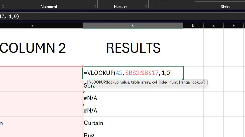
11. Add a close parenthesis to end the formula. Your formula should look something like =VLOOKUP(A2, $B$2:$B$17, 1,0). A2 and $B$2:$B$17 will be different for you, though.

Marinel Sigue/SlashGear

Hit Enter to apply the formula. To apply the formula to the rest of the rows, grab the small square in the bottom-right corner of the cell (fill handle) and drag it to the end of the column to fill the entire column. The third column should now be filled with results. If a value in the first column matches one in the second column, that same value will appear as a result. If you get a #N/A error instead, it means the value isn't in the second column.

If you need to compare two columns in Excel row-by-row instead of the entire column at once, use comparison operators. They check the values in each row and output TRUE if the data are the same or FALSE if the data don't match. Follow these steps to use comparison operators in Excel:

1. Under a new column next to your existing data, put an equal sign (=).
2. Then, click on the first row of the first column.
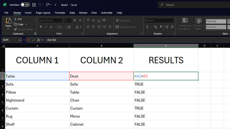
3. To check whether the data match, type another equal sign.
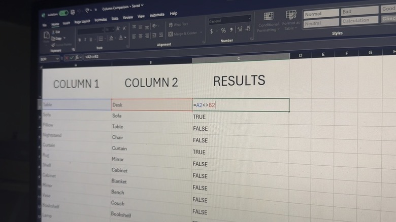
4. To check whether the data is different, enter a not equal sign (<>).
5. Click on the first row of the second column to complete the operation.

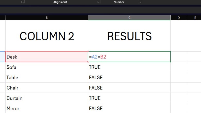
If you're checking for matching data, the first row of the third column should look like =A2=B2. Otherwise, it should be =A2<>B2.

Marinel Sigue/SlashGear

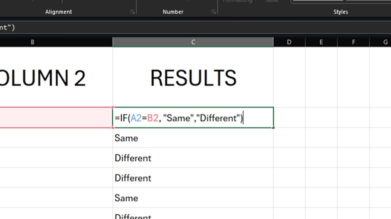
Press Enter to save the formula, and you should see a TRUE or FALSE value in the cell. Apply the same formula to the rest of the column by grabbing and dragging the fill handle in the first row of the results column. If you want to show custom words instead of the default TRUE or FALSE, you can add an IF function to your formula to set your own result. The formula for checking whether the data are similar then becomes =IF(A2=B2, "Same","Different"), where Same is the result if A2=B2 is true and Different is the result if A2=B2 is false.

Marinel Sigue/SlashGear

You'll have to drag the formula cell again to the bottom of the column to apply this new IF formula to all the other rows.